Chapter 2 · Part I — Curves, tropicalised

A Conic Is a Line That Got Caught Twice

A conic is a line that got caught twice: weights are memory, and coefficients subdivide the triangle.

11 min read

Chapter 1 ended with a cliffhanger: min(2x, 2y, 0) draws exactly the same set of points as the tropical line, and yet it isn’t the same curve. This chapter names the missing ingredient — weight — and then meets the first real family of curves: the conics. Along the way we’ll learn how coefficients reach into the Newton polygon and subdivide it, why one conic is a line in disguise and another is a tree pretending to be a circle, and where the cycle we keep hoping for is hiding. (Not here. We checked. Twice.)

First, a one-variable warm-up, because it’s the fastest way to see weights being born.

2.1 Roots, in one variable: the missing root didn’t vanish, it collided

In one variable, a tropical “curve” is a set of points on a line: the roots of f(x) = min(2x, x + 1, 0), where the min is attained at least twice. There are three terms, so there are three candidate tie points. Evaluate all three terms at each:

Candidate	Why it’s a candidate	Values (2x, x+1, 0)	Root?
x = 1	2x = x + 1	(2, 2, 0)	no — min 0 attained once
x = 0	2x = 0	(0, 1, 0)	yes
x = −1	x + 1 = 0	(−2, 0, 0)	no — min −2 attained once

Only x = 0 is a root. But this is a degree-2 polynomial! The classical fundamental theorem of algebra promises two roots, counted with multiplicity. Is the tropical version just… lying?

No — it’s counting differently. Look at the graph of the min function. For x → −∞ it follows the term 2x, slope 2. For x → +∞ it follows the term 0, slope 0. At the root x = 0 the slope jumps from 2 to 0 — a jump of size 2. That jump is the multiplicity:

A tropical root’s multiplicity is the size of the slope jump at it — equivalently, the lattice length of the edge it is dual to in the Newton polygon (here the edge from exponent 0 to exponent 2).

So x = 0 is a root of multiplicity 2, and 2 = 2: the tropical fundamental theorem of algebra holds — with multiplicity. The second root didn’t vanish. It collided with the first, and the collision left a number behind. That number is our first weight.

2.2 Weights: edges remember their duals’ lengths

Now back to two variables. Every edge of a tropical curve is dual to an edge of (a subdivision of) the Newton polygon, per Chapter 1. Edges of the curve carry a positive integer weight:

Weight of a curve edge = lattice length of its dual polygon edge — the number of primitive steps in it. An edge from (0,0) to (2,0) has lattice length 2. An edge from (0,0) to (1,1) has lattice length 1 (it’s already primitive).

And balancing, Chapter 1’s (0,1) + (1,0) + (−1,−1) = 0, upgrades to its real form:

Weighted balancing: at every vertex, Σᵢ wᵢ·vᵢ = 0, where vᵢ are the primitive directions of the edges at the vertex and wᵢ their weights.

Chapter 1’s line had all weights 1, so the weights were invisible. Now solve the Chapter 1 cliffhanger: min(2x, 2y, 0) has exponents (0,0), (2,0), (0,2) — a triangle with every edge of lattice length 2. Same three ray directions, but every weight is 2:

2·(0,1) + 2·(1,0) + 2·(−1,−1) = (0, 0) ✓ (still balances, of course)

Same picture, different curve: the tripod, counted twice. Tropical geometry refuses to forget multiplicity, and weights are how it remembers. Keep them in your pocket — a famous counting theorem in Part II is basically bookkeeping of exactly these numbers.

2.3 The degenerate conic: a doubled line

A conic is a degree-2 curve: all terms c + ix + jy with i + j ≤ 2 — six lattice points, the Newton triangle with corners (0,0), (2,0), (0,2). Start with the laziest coefficients of all: every c = 0.

f(x, y) = min(2x, 2y, x+y, x, y, 0)

No coefficient distinguishes any point of the triangle, so the polygon doesn’t subdivide: one cell, dual to one vertex. Three boundary edges, each of lattice length 2, give three rays of weight 2. The “conic” is the doubled tropical line of §2.2.

Postcard from classical geometry. This is the tropical shadow of a non-reduced conic: classically, (x + y + 1)² = 0 is “a line, doubled” — the equation remembers being squared even though the solution set is just a line. Tropicalisation preserves exactly that memory, as weights. The bare set forgets; the weighted graph doesn’t. This is why tropical curves are weighted graphs and not just graphs, full stop.

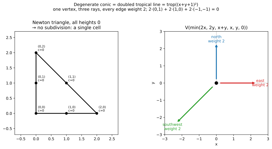
Figure 2.1 — All coefficients zero: no subdivision, one vertex, three rays of weight 2.

2.4 Coefficients lift, and the polygon subdivides

Now give the terms distinct coefficients — “generic” heights. Take

c(i, j) = i² + j²,   except c(1, 1) = 2.5 instead of 2.

Here’s the mechanism, and it’s worth learning properly because the whole book runs on it:

1. Lift each lattice point (i, j) up to height c(i, j) in 3D.
2. Take the lower convex hull of the lifted points — imagine resting the cloud of points on a table, and looking at the faces you can see from below.
3. Project those lower faces back down. The Newton polygon comes back cut into pieces: a regular subdivision.

Why the bump at (1,1)? At height exactly 2, the four lifted points (0,0,0), (1,0,1), (0,1,1), (1,1,2) all lie on the plane z = x + y — a four-way tie, dual to one 4-valent vertex. Raising (1,1) slightly breaks the tie and picks a diagonal, giving the clean trivalent picture below. (Lowering it would pick the other diagonal. Either way: a choice was hiding in the flat spot, and the coefficients make it.)

Our subdivision has four unit triangles (area ½ each — they exactly tile the area-2 triangle):

Face (lattice points)	Dual vertex
(0,0), (1,0), (0,1)	(−1, −1)
(1,0), (2,0), (1,1)	(−3, −1.5)
(0,1), (0,2), (1,1)	(−1.5, −3)
(1,0), (0,1), (1,1)	(−1.5, −1.5)

Each face’s vertex is where its three terms tie for the global minimum — the chapter’s program checks that, exactly, for all four.

2.5 Anatomy of the smooth conic

Duality now produces a real graph, not a tripod:

• 4 vertices, one per triangle.
• 3 bounded edges, dual to the 3 subdivision edges shared by two triangles. All three are incident to the central face (1,0),(0,1), (1,1) — the bounded graph is a star, hence a tree.
• 6 rays, dual to the 6 boundary edges, all of weight 1: two in each of the three Chapter-1 directions.
• Balancing holds at all 4 vertices (checked in the full program from the subdivision data).

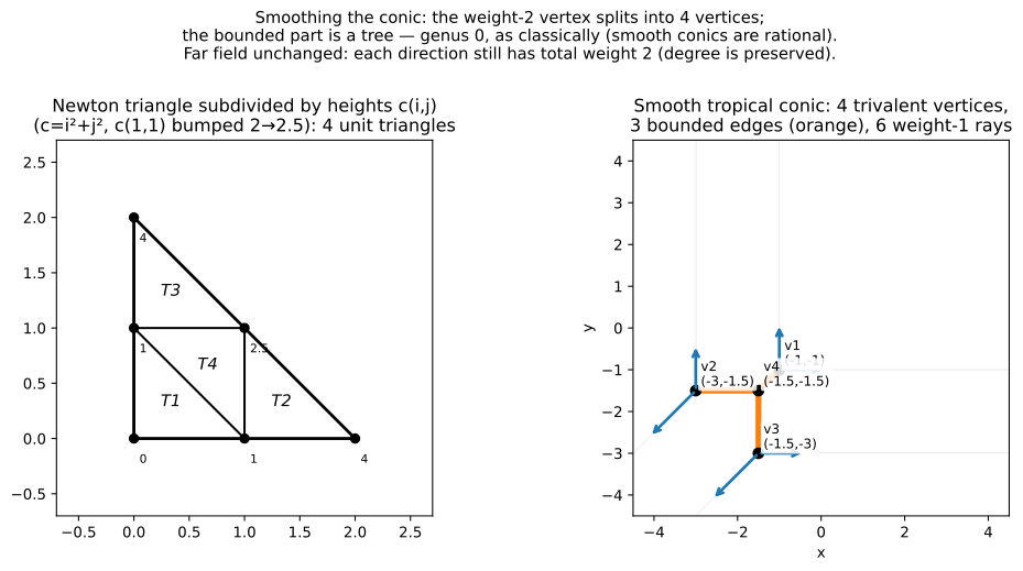
Figure 2.2 — Subdivided Newton triangle (left) and the smooth tropical conic (right): 4 vertices, 3 bounded edges, 6 rays. No cycle.

Notice the far field: two rays in each direction, total weight 2 per direction — exactly the degenerate conic’s weights. Smoothing resolved the fat vertex into four thin ones, but from far away nothing changed. Degree is a far-field invariant, and deformation can’t touch it. File that away; Part II’s counting theorems are this observation, weaponised.

2.6 Where’s the cycle? (An honest non-appearance)

A classical smooth conic is a sphere; its tropical shadow should have “sphere-ness” about it. The combinatorial version of that number is the genus of the graph:

g = E − V + 1     (bounded edges − vertices + 1, for a connected graph)

For our conic: g = 3 − 4 + 1 = 0. The bounded part is a tree. There is no cycle. And here’s the theorem that explains why there couldn’t be one:

For a smooth tropical plane curve of degree d, g = the number of interior lattice points of the Newton triangle = (d−1)(d−2)/2.

The degree-2 triangle’s lattice points are all on its boundary — it has zero interior points — so every smooth tropical conic has genus 0, matching the classical fact that a smooth conic is rational (a sphere, genus 0). The formula’s first interesting value is at d = 3: (2·1)/2 = 1. One interior point. One cycle. Next chapter.

Honest Box — a prediction that failed, on the record. The study notes written the night before this computation predicted the smooth conic “acquires a cycle.” It’s preserved in the notes as a correction, because it’s the instructive kind of wrong: the intuition “smoothing creates topology” is fine, but the interior-point count was checkable in advance and says genus 0 outright. House rule, restated: count first, then hope.

2.7 Closing Chapter 1’s Honest Box: the rays, from the picture alone

Chapter 1 confessed that its balancing check used hand-derived ray directions. The full Day 1 program closes that gap: it takes the sampled tie-mask — just the bitmap of the curve — clusters the far-field points by angle, fits each cluster’s direction by PCA, snaps to the nearest primitive integer vector, and re-checks balancing on the inferred directions. Result, for both conics in this chapter: snap error 0.00° on every cluster, inferred directions balance to (0, 0). The smooth conic’s six inferred rays are two each of (0,1), (1,0), (−1,−1) — the far-field claim of §2.5, recovered from pixels. The picture now testifies on its own behalf.

2.8 The whole chapter, as a program

from fractions import Fraction as F

# --- warm-up: tropical roots of min(2x, x+1, 0) ---
def wvals(x): return (2*x, x+1, 0)
roots = []
for cand in [F(1), F(0), F(-1)]:       # the three pairwise tie points
    v = wvals(cand)
    if v.count(min(v)) >= 2:
        roots.append(cand)
assert roots == [F(0)], roots          # only x=0 is a root
# multiplicity: slope of the min-graph jumps 2 -> 0 at x=0, a jump of 2
assert 2 - 0 == 2

# --- the degenerate conic: all coefficients 0 ---
rays_w = [((0, 1), 2), ((1, 0), 2), ((-1, -1), 2)]  # (direction, weight)
bal = (sum(w*d[0] for d, w in rays_w), sum(w*d[1] for d, w in rays_w))
assert bal == (0, 0), bal              # weighted balancing: sum w_i v_i = 0

# --- the smooth conic: heights c(i,j)=i^2+j^2, c(1,1) bumped 2 -> 5/2 ---
PTS = [(0,0), (1,0), (2,0), (0,1), (1,1), (0,2)]
C = {(0,0): F(0), (1,0): F(1), (2,0): F(4),
     (0,1): F(1), (1,1): F(5,2), (0,2): F(4)}
def val(p, x, y): return C[p] + p[0]*x + p[1]*y

FACES = [{(0,0), (1,0), (0,1)}, {(1,0), (2,0), (1,1)},
         {(0,1), (0,2), (1,1)}, {(1,0), (0,1), (1,1)}]
VERTS = [(F(-1), F(-1)), (F(-3), F(-3,2)), (F(-3,2), F(-3)), (F(-3,2), F(-3,2))]

def area2(face):
    (x1,y1),(x2,y2),(x3,y3) = sorted(face)
    return abs(x1*(y2-y3) + x2*(y3-y1) + x3*(y1-y2))
for face, (x, y) in zip(FACES, VERTS):
    assert area2(face) == 1                       # unit triangle (area 1/2)
    vals = {p: val(p, x, y) for p in PTS}
    m = min(vals.values())
    assert {p for p, v in vals.items() if v == m} == face  # face ties, globally
# the 4 unit triangles exactly tile the degree-2 triangle (area 2)
assert sum(area2(f) for f in FACES) == 4           # in doubled-area units: 2*2

# bounded edges = subdivision edges shared by two faces
from itertools import combinations
bounded = []
for a, b in combinations(range(4), 2):
    shared = FACES[a] & FACES[b]
    if len(shared) == 2:
        bounded.append((a, b))
assert sorted(bounded) == [(0, 3), (1, 3), (2, 3)]  # a star: a tree
genus = len(bounded) - len(FACES) + 1
assert genus == 0
interior = [p for p in PTS if p[0] > 0 and p[1] > 0 and sum(p) < 2]
assert interior == []                              # no interior lattice points
print("Chapter 2: all assertions pass. Weighted balancing:", bal, "| genus:", genus)

Chapter 2: all assertions pass. Weighted balancing: (0, 0) | genus: 0

Honest Box — what this program checks. The compact program takes the subdivision (the four faces) as given and verifies everything downstream exactly: unit areas, tiling, the global tie at each dual vertex, the bounded-edge structure, genus, weighted balancing of the degenerate conic. The subdivision itself — lower hull of the lifted points, via scipy’s ConvexHull — plus balancing at all four vertices and the mask inference of §2.7, are in the full program (ch02_tropical_conic.py, the study’s Day 1 code), which asserts them all.

2.9 Try It

1. Triple line. Predict, before computing: the rays and weights of min(3x, 3y, 0), and check weighted balancing. What classical object is it the shadow of?
2. Check a vertex by hand. At the smooth conic’s vertex (−3, −1.5), evaluate all six terms c + ix + jy. Which three tie, and what is the minimum value?
3. Count ahead. List the interior lattice points of the degree-4 Newton triangle (i, j ≥ 0, i + j ≤ 4, strict interior). How many are there, and what genus does §2.6’s formula predict for a smooth tropical quartic?

Answers

• 1. Same three directions, every weight 3 (boundary edges now have lattice length 3); 3·(0,1) + 3·(1,0) + 3·(−1,−1) = (0,0). Shadow of a triple line — a non-reduced “conic-plus” (a degree-3 line counted three times).
• 2. Values: (0,0) ↦ 0; (1,0) ↦ 1−3 = −2; (2,0) ↦ 4−6 = −2; (0,1) ↦ 1−1.5 = −0.5; (1,1) ↦ 2.5−3−1.5 = −2; (0,2) ↦ 4−3 = 1. The face (1,0), (2,0), (1,1) ties at −2, and nothing undercuts it.
• 3. Interior points: (1,1), (1,2), (2,1) — 3 points, genus 3. (Keep this; a later chapter builds that quartic and finds three cycles, arranged in a way worth the wait.)

What we learned

• Multiplicity is a slope jump; in two variables it becomes weight = lattice length of the dual edge, and balancing is Σ wᵢvᵢ = 0.
• Coefficients lift the Newton polygon’s points; the lower hull projects to a subdivision; faces ↔ vertices, shared edges ↔ bounded edges, boundary edges ↔ rays.
• A smooth conic’s bounded graph is a tree: genus 0, because the degree-2 triangle has no interior lattice points.
• Smoothing redistributes vertices but conserves the far field: degree is read off at infinity, in total ray weights.

Next

Degree 3. The triangle grows one interior lattice point, (1,1) — and its six surrounding triangles will dualise into something the conic couldn’t have: a cycle, the tropical shadow of a torus. Chapter 3 builds the tropical elliptic curve and teaches the bounded graph to hold water.

---

Source & provenance: Day 1 (2026-10-11) of the tropical geometry study — code hidden_files/code/day01_tropical_conic.py (run log hidden_files/day01-run.log), figures files/figures/day01-degenerate-conic.png and day01-smooth-conic.png, study log Day 1 entry. The code in §2.8 was executed and passed on 2026-10-30.

Chapter code

The full program behind this chapter, as a download: ch02_tropical_conic.py. The inline listing in the chapter is the compact, self-checking version.