Chapter 1 · Part I — Curves, tropicalised

Addition Is Min, Multiplication Is Plus (and a Line Is Not a Line)

Break arithmetic on purpose — and watch a line fall apart into three rays that balance.

12 min read

Welcome! In this book we are going to do something slightly rude to arithmetic, and then watch geometry survive it — changed, simplified, and frankly better-looking.

Ordinary geometry starts with equations like

x + y = 0

and draws you a line. We are going to keep the equation, change what the symbols mean, and draw it again. The line will fall apart into three rays stuck together at a point. Strangely, almost everything that mattered about the line — its degree, its direction at infinity, its genus (zero, in case you were worried) — will still be there, written in the rays.

That’s tropical geometry: algebraic geometry after a very lossy, very honest compression. Curves become graphs. Smooth things become combinatorial things. And — this is the part that makes the whole book possible — you can compute all of it, with short programs, and check every claim as you go.

No algebraic geometry is assumed. If you know what a polynomial is and you’ve seen a coordinate plane, you have the prerequisites. Let’s break arithmetic.

1.1 Two new operations, zero new numbers

Take the ordinary real numbers, plus one extra value, infinity (∞). Now define two operations and give them grand names:

• Tropical addition: a ⊕ b = min(a, b) — “add” by taking the smaller.
• Tropical multiplication: a ⊗ b = a + b — “multiply” by adding, ordinarily.

That’s it. That’s the tropical semiring. Some quick experiments, the way you’d poke a new programming language at a REPL:

3 ⊕ 7  = min(3, 7)  = 3
3 ⊗ 7  = 3 + 7      = 10
5 ⊕ 5  = 5
9 ⊕ ∞  = 9        (∞ is the identity for ⊕: min(∞, a) = a)
9 ⊗ 0  = 9        (0 is the identity for ⊗: 0 + a = a)

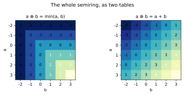
The whole semiring at a glance, for small values of “whole.” Left: ⊕ — read the idempotence straight off the diagonal, where a ⊕ a = a. Right: ⊗, ordinary addition wearing a costume.

Everything should feel almost normal, and then one thing should itch: 5 ⊕ 5 = 5. In ordinary arithmetic, adding a thing to itself makes it bigger. Tropically, a ⊕ a = a for every a. This property is called idempotence, and it’s the first sign we’re not in a field any more. A close relative of the itch: there is no tropical subtraction. Given min(a, b), you can’t recover what got thrown away. Information is destroyed on purpose. Hold onto that — the whole subject lives in what survives the destruction.

The operations do still cooperate, in exactly the way that makes polynomials work:

a ⊗ (b ⊕ c)  =  a + min(b, c)  =  min(a + b, a + c)  =  (a ⊗ b) ⊕ (a ⊗ c)

Multiplication distributes over addition. So we can build tropical polynomials: expressions made from variables and constants using only ⊕ and ⊗. And here is what one looks like when you unfold the definitions. Take the tropical polynomial “x ⊕ y ⊕ 0”. Unfolding:

x ⊕ y ⊕ 0  =  min(x, y, 0)

A tropical polynomial in two variables is always a minimum of terms, and each term has the shape

c + i·x + j·y

for a constant c and non-negative integers i, j — the exponents. (Why do exponents show up as multipliers? Because tropically, x ⊗ x means x + x, which in ordinary notation is 2x. Powers become multiples. Multiplication became addition, so exponentiation became multiplication. Everything moves down one rung of the ladder.)

A note on conventions. Half the literature uses min-plus, as we do; the other half uses max-plus. They’re mirror images (negate everything) and both are called “tropical.” This book is min-plus throughout, and will wave a small flag whenever a source we’re following uses the other side of the mirror.

1.2 A curve is where the minimum is attained twice

Now the definition the entire book hangs on — it’s one sentence:

The tropical curve of a tropical polynomial is the set of points where the minimum is attained at least twice.

Why twice? Think about what a single winning term means: at such a point, one term is strictly smaller than all the others, and it stays the winner in a whole little neighbourhood — nothing interesting happens there; the polynomial is locally just one smooth sheet, c + i·x + j·y. The interesting places are where the lead changes hands, where two terms tie for smallest. Ordinary algebraic geometry finds curves where a polynomial equals zero. Tropical geometry finds curves where a polynomial can’t decide which term is smallest. The tie locus is the curve.

Let’s compute our first one, by hand, completely.

The tropical line: f(x, y) = min(x, y, 0), three terms: the value x, the value y, and the value 0. Pick some points and score them:

Point	Terms (x, y, 0)	Min attained	On the curve?
(0, 2)	(0, 2, 0)	twice: x-term and 0	yes
(2, 0)	(2, 0, 0)	twice: y-term and 0	yes
(−2, −2)	(−2, −2, 0)	twice: x-term and y	yes
(1, 1)	(1, 1, 0)	once: only 0	no
(−1, 1)	(−1, 1, 0)	once: only x	no
(1, −1)	(1, −1, 0)	once: only y	no

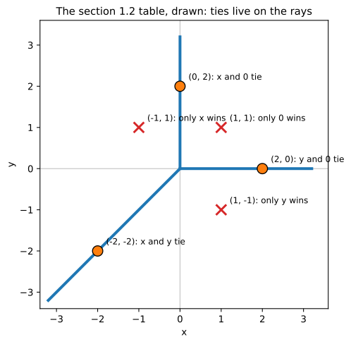
The table, drawn. Orange dots tie, and sit exactly on the rays; red crosses have a single winner, and sit in the open regions between them. Every point in the plane is one or the other — that dichotomy is the curve.

Now let’s find all the ties, not just at our sample points.

• Where do the x-term and the 0-term tie, and win? Need x = 0 and 0 ≤ y (so the y-term doesn’t undercut them). That’s the ray straight up from the origin: points (0, t), t ≥ 0.
• Where do y and 0 tie, and win? Need y = 0 and 0 ≤ x. The ray straight right: (t, 0), t ≥ 0.
• Where do x and y tie, and win? Need x = y and x ≤ 0 (so the 0-term doesn’t win alone). The ray down-left: (t, t), t ≤ 0.

And everywhere else, exactly one term wins outright, so there is no more curve. The plane is divided into three regions — one where 0 wins (the first quadrant’s interior), one where x wins, one where y wins — and the curve is exactly the border system between them.

A line is a tripod. Three rays from a single vertex at the origin, pointing in the directions

(0, 1)    north
(1, 0)    east
(−1, −1)  southwest

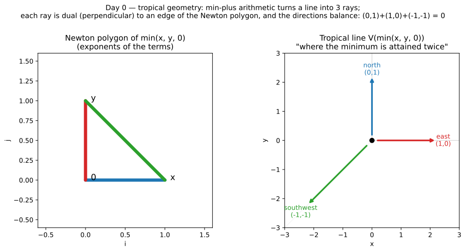
Figure 1.1 — Left: the Newton polygon (next section). Right: the tropical line V(min(x, y, 0)). Three rays, one vertex, no line in sight.

Try It 1.1. For each point, evaluate all three terms and decide: on the curve or not? (a) (2, 2) (b) (−3, 0) (c) (0, −5) (d) (−1, −1). Two of these are traps: they sit on the lines containing rays but not on the rays themselves. Answers at the end of the chapter.

1.3 The Newton polygon: the curve’s shadow, drawn in advance

Look at the exponents of our three terms: x has exponent (1, 0), y has (0, 1), and the constant 0 has (0, 0). Plot those three points and take their convex hull — stretch a rubber band around them. You get a triangle. This is the Newton polygon of the polynomial, and it knows the curve’s shape before we compute anything:

Duality. Each edge of the Newton polygon corresponds to one ray of the tropical curve. The ray is perpendicular to its edge and points like the edge’s inward normal.

Check it against Figure 1.1:

• Bottom edge, (0,0)–(1,0): horizontal edge, inward normal (0, 1) → the north ray. ✓
• Left edge, (0,0)–(0,1): vertical edge, inward normal (1, 0) → the east ray. ✓
• Hypotenuse, (1,0)–(0,1): direction (−1, 1); perpendicular to it is (−1, −1) (dot product: (−1)(−1) + (1)(−1) = 1 − 1 = 0 ✓), pointing inward → the southwest ray. ✓

Three edges, three rays. This is the first appearance of the book’s central bargain: continuous geometry on one side, finite combinatorics on the other, and a dictionary between them. In Chapter 2 the polygon will get subdivided by the coefficients, and that’s when curves start growing vertices, bounded edges, and eventually cycles. For now, notice we could have drawn the right-hand picture from the left-hand one with a ruler and the duality rule alone.

1.4 Balancing: why these graphs deserve to be called curves

One more condition, the most important one in the book. Add the three ray directions:

(0, 1) + (1, 0) + (−1, −1) = (0, 0)

They balance. This is not a coincidence of our example; it is a theorem-shaped fact about every tropical curve, at every vertex (in general: Σ wᵢ·vᵢ = 0, where wᵢ are positive integer weights we’ll meet in Chapter 2 — here all weights are 1). The rays pull in their directions with their weights, and the total pull is zero, like forces in equilibrium, or currents at a node satisfying Kirchhoff’s law.

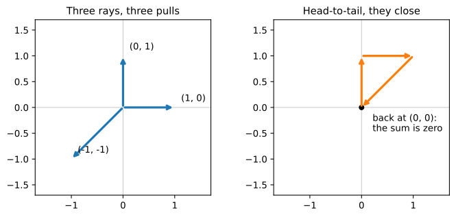
Left: the three ray directions as pulls from the vertex. Right: the same three vectors head-to-tail. They close — that loop closing is what (0, 1) + (1, 0) + (−1, −1) = (0, 0) looks like.

Balancing is the discrete soul of the subject. A random tripod is just a graph; a balanced graph is a curve — it’s the condition that lets these pictures carry intersection theory, genus, Jacobians, and curve-counting, all of which are coming. Whenever this book draws you a graph and calls it a curve, the receipt is a balancing sum that comes out to zero.

1.5 The whole chapter, as a program

Here is everything above, as runnable Python. The assertions are the chapter’s claims — run it, and if it prints the final line, the tropical line is what we said it is.

INF = float("inf")

def tadd(a, b): return min(a, b)   # tropical addition
def tmul(a, b): return a + b       # tropical multiplication

assert tadd(3, 7) == 3
assert tmul(3, 7) == 10
assert tadd(5, 5) == 5             # idempotent: a (+) a = a
assert tmul(0, 9) == 9             # 0 is the tropical multiplicative identity
assert tadd(INF, 9) == 9           # INF is the tropical additive identity

def terms(x, y): return (x, y, 0)  # the three terms of min(x, y, 0)

def on_curve(x, y):
    vals = terms(x, y)
    return vals.count(min(vals)) >= 2

for p in [(0, 2), (3, 0), (-2, -2), (0, 0)]:
    assert on_curve(*p), p         # one point on each ray, plus the vertex
for p in [(1, 1), (-1, 1), (1, -1), (2, -3)]:
    assert not on_curve(*p), p     # one winner only -> not on the curve

rays = [(0, 1), (1, 0), (-1, -1)]
bal = (sum(r[0] for r in rays), sum(r[1] for r in rays))
assert bal == (0, 0), bal           # balancing

print("Chapter 1: all assertions pass. Balancing sum:", bal)

Chapter 1: all assertions pass. Balancing sum: (0, 0)

(The full plotting program that draws Figure 1.1 — grid, tie-mask, Newton polygon, colour-matched dual edges — ships with the chapter as ch01_tropical_line.py. It’s the study’s Day 0 program, lightly renamed.)

Honest Box — what this program does and doesn’t prove. The tie checks and the balancing sum are exact. But the ray directions in the code are the ones we derived by hand; the program sums those, it doesn’t extract them from the picture. Inferring the rays from the plotted mask alone — no hand-fed answers — is a stricter test, and it’s a real exercise in the study this book is built from. It gets closed in Chapter 2, where the rays are recovered from the bitmap and balance still comes out to (0, 0). We tell you this now because the house rule of this book is: a check is only worth what it actually checks.

1.6 Try It

1. (Warm-up, from §1.2’s table.) Redo Try It 1.1(c) slowly: at (0, −5), which term wins, and by how much? What goes wrong with the guess “x = 0 is the north ray”?
2. Move the vertex. Consider g(x, y) = min(x, y, 1). Find where all three terms tie. Predict the three rays (directions and starting points) using duality before evaluating anything. Then check three points with the tie test: does the southwest ray pass through the origin?
3. A teaser for Chapter 2. Consider min(2x, 2y, 0). Show that, as a set of points, its curve is identical to the tropical line’s. And yet — it is not the same curve. What’s missing from the picture that could tell them apart? (Chapter 2’s first word is the answer.)

Answers

• Try It 1.1. (a) (2, 2): terms (2, 2, 0) — 0 wins alone, off. (b) (−3, 0): terms (−3, 0, 0) — x wins alone, off (the east ray needs x ≥ 0). (c) (0, −5): terms (0, −5, 0) — y wins alone, off (the north ray needs y ≥ 0). (d) (−1, −1): terms (−1, −1, 0) — tie, on (southwest ray).
• Try It 1.6.2. All three tie when x = y = 1: the vertex moves to (1, 1). Rays: north from (1, 1) along x = 1, y ≥ 1; east along y = 1, x ≥ 1; southwest along x = y ≤ 1 — same directions as before (the Newton polygon didn’t change, only the constants did), and yes, the southwest ray passes through (0, 0), since min(0, 0, 1) = 0 is attained twice.
• Try It 1.6.3. 2x = 2y iff x = y, 2x = 0 iff x = 0, etc. — every tie condition is the old one scaled, so the set is identical. The missing ingredient is weight: that curve is a line counted twice. Chapter 2 makes weights precise — and shows a conic that is secretly exactly this.

What we learned

• Tropical arithmetic: ⊕ is min, ⊗ is plus; the semiring is idempotent and has no subtraction, and polynomials still work.
• A tropical curve is where a tropical polynomial’s minimum is attained at least twice.
• The tropical line is three rays, each dual to an edge of the Newton polygon, and their directions balance: they sum to zero.

Next

Chapter 2 raises every exponent: the conic min(2x, 2y, x+y, x, y, 0). With flat coefficients it’s a doubled line wearing a conic’s clothes. With generic coefficients, its Newton triangle subdivides, the tripod sprouts three extra vertices — and we’ll ask the question whose answer is the genus: where’s the cycle?

---

Source & provenance: this chapter converts Day 0 (2026-10-10) of the tropical geometry study — code hidden_files/code/day00_tropical_line.py, figure files/figures/day00-tropical-line.png, study log Day 0 entry. All code in §1.5 was executed and passed on 2026-10-30; one assertion in an early draft of the Try It answers was caught by that run (the southwest ray of min(x, y, 1) does pass through the origin) and the answer above is the corrected one. The three extra figures (the operations tables, the six points drawn, the balancing arrows) were added 2026-11-01: code hidden_files/code/ch01_extra_figures.py, asserted the same way — classification, idempotence diagonal, and the balancing sum are all checked in code before anything is drawn.

Chapter code

The full program behind this chapter, as a download: ch01_tropical_line.py. The inline listing in the chapter is the compact, self-checking version.