Chapter 11 — The Petersen Graph Is a Moduli Space · Learn You a Tropical Geometry for Great Good!

Chapter 10 ended with a tripod: trop Gr(2,4), modulo its lineality, is a tropical line, and its three rays are the three ways to resolve a 4-leaf star tree. This chapter takes one more leaf. The punchline is stated up front, because it is hard to believe otherwise:

The space of trees on five leaves — the tropical Grassmannian Gr(2,5) after its three prime reductions — is the Petersen graph.

The Petersen graph is combinatorics’ favourite counterexample: the smallest snark seed, nonplanar, hypohamiltonian, the graph that breaks naive conjectures. Here it is not a counterexample to anything. It is a moduli space: its vertices are the ways a 5-leaf tree can begin to resolve, and its edges are the fully resolved trees themselves. Everything below is Speyer– Sturmfels, “The tropical Grassmannian” (arXiv:math/0304218), Example 3.3 and Theorem 3.4, computed end to end.

11.1 First, the reductions: why a graph at all?

The full fan Gr(2,5) lives in ℝ^{C(5,2)} = ℝ^{10}; its maximal cones have dimension (n−d)d + 1 = 7. Speyer– Sturmfels peel off the uninteresting directions in three steps (§3 of the paper):

G′ = the fan modulo ℝ·(1,…,1) — dimension 6;
G″ = the fan modulo image(φ), where φ(a)_{ij} = a_i + a_j is Chapter 10’s pendant-edge freedom — dimension (d−1)(n−d−1) = 2. The bookkeeping, stated once with its ambients: image(φ) — the fan’s lineality — is 5-dimensional in ℝ¹⁰ (φ is injective for n ≥ 3; the program asserts rank 5), so a maximal cone splits as 7 = 5 + 2, lineality plus genuine fan. And (1,…,1) = φ(½·(1,…,1)) already lies in image(φ), so the G′ step is redundant inside the G″ step, not a separate direction;
G‴ = G″ intersected with the unit sphere — maximal face dimension nd − n − d² = 1.

Dimension 1 means: a graph. Its vertices are the rays of G″, its edges the 2-dimensional cones. The rest of the chapter names those rays and cones — and then checks that the graph they form really is Petersen’s, by its invariants, not by its silhouette.

11.2 Splits: the vertices

A split of the leaf set {1,…,5} is a partition A | A^c with both sides of size at least 2 — one internal edge of a tree, recording which leaves lie on each side. For n = 5 every split is 2|3, so a split is determined by its 2-side, and there are

2^{5−1} − 5 − 1 = 10

of them: 12, 13, 14, 15, 23, 24, 25, 34, 35, 45 (each read as A | A^c). Theorem 3.4 says the vertices of tree space T_n are exactly the splits, for every n. Ten vertices is the Petersen graph’s first invariant — but ten vertices is also just a number. The edges decide.

Two splits can occur in one tree exactly when they are compatible: the paper’s condition (4) — for splits {A, A^c} and {B, B^c}, one of A ⊆ B, A ⊆ B^c, A^c ⊆ B, A^c ⊆ B^c holds. For 2|3 splits the program checks all 45 pairs and finds condition (4) collapses to something you can see:

Two 2|3 splits are compatible iff their 2-sides are disjoint.

So the compatibility graph has as vertices the 2-subsets of a 5-set, joined when disjoint — which is the definition of the Kneser graph KG(5,2). And KG(5,2) is the classical second construction of the Petersen graph. (A third name for the same graph, worth one sentence because it is where Aut = S₅ comes from: it is the complement of the line graph L(K₅) — the vertices of L(K₅) are the edges of K₅, i.e. the 2-subsets, adjacent exactly when they share a vertex, so complement adjacency is exactly disjointness. The program checks this pair by pair.) The identification is therefore not an analogy: build the graph from splits and you have built Petersen’s graph, vertex for vertex, edge for edge. The next section proves the drawing honest by computing the invariants Petersen is famous for.

11.3 Petersen, proved Petersen

Predict first. If the compatibility graph is Petersen, it must be 3-regular with 15 edges (each 2-set is disjoint from exactly the three 2-subsets of its 3-element complement), have girth 5 — no triangles (three pairwise disjoint 2-sets would need six leaves) and no 4-cycles — diameter 2, and be nonplanar. The program asserts each of these, several of them twice:

10 vertices, 15 edges, 3-regular, connected, diameter 2.
Girth exactly 5: BFS from every vertex, and independently by brute force — 0 triangles, 0 ordered 4-cycles, and an explicit 5-cycle 12–34–15–23–45–12.
Chromatic number 3 (backtracking; > 2 already follows from the odd cycle) and independence number 4.
Nonplanar, by the girth-5 Euler bound: a planar graph of girth at least 5 has E ≤ (5/3)(V−2) = 13.33…, but 15 > 13.33….
Symmetry: S₅, permuting the leaves, induces 120 distinct automorphisms, transitive on vertices and on edges. (The classical statement is Aut = S₅; the program verifies S₅ ≤ Aut, which is the direction the moduli story needs — relabelling leaves really is a symmetry of tree space.)
Hypohamiltonian: brute-force search finds no Hamiltonian cycle, while deleting any one vertex leaves a graph that does have one — asserted for all ten deletions, not just one up to symmetry.

One more number ties the graph back to the theorem. Theorem 3.4 says T_n has the homotopy type of a bouquet of (n−2)! spheres of dimension n−4. For n = 5 those are circles, and a graph’s circle count is its cycle rank — its first Betti number b₁:

E − V + 1 = 15 − 10 + 1 = 6 = (5−2)!.

Six circles’ worth of homotopy, on the nose. The same Euler-characteristic bookkeeping checks at the neighbours: T₄ has χ = 3 = 1 + 2 (a wedge of two copies of S⁰ — three points), and T₆ has χ = 25 − 105 + 105 = 25 = 1 + 24 (a wedge of 24 copies of S²; §11.7).

A facet of T₅ is a maximal compatible family of splits — a maximal clique of the compatibility graph. The program finds the maximal cliques are exactly the 15 edges themselves: no three splits are pairwise compatible (three pairwise disjoint 2-sets again — six leaves, impossible). So every facet has size 2 = n − 3, and:

A facet is a pair of disjoint splits, and a pair of disjoint splits is a trivalent tree on five leaves — two internal edges, three internal vertices, five pendants.

The count agrees with the theorem’s (2n−5)!! = 5!! = 15 trivalent trees, and every split lies in exactly 3 trees (its three disjoint partners — 3-regularity again, read as incidence). Panel B of Figure 11.1 draws one facet as the tree it is: cherries {1,2} and {4,5}, leaf 3 attached at the middle vertex.

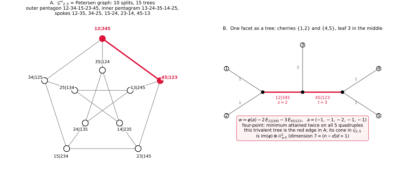
The Petersen graph as tree space: vertices labelled by splits, the red edge drawn beside it as the trivalent tree it is

Figure 11.1 — A: G‴_{2,5} in the classic pentagon/pentagram drawing; vertices are splits A|A^c, edges are trivalent trees. Outer pentagon 12–34–15–23–45–12 (the explicit 5-cycle of §11.3), inner pentagram 13–24–35–14–25, spokes 12–35, 34–25, 15–24, 23–14, 45–13. B: the red edge {12|345, 45|123} as a tree — cherries {1,2} and {4,5}, leaf 3 central — with the worked decomposition w = φ(a) − 2·E_{12|345} − 3·E_{45|123}, a = (−1,−1,−2,−1,−1), re-asserted in the figure script before rendering.

So the Petersen graph’s edges are not glue or decoration. Each edge is a tree — the complete, fully resolved object of which its two endpoint splits are the two internal edges.

11.5 Back at fan level: cones, membership, initial forms

G‴ is the shadow; the fan Gr(2,5) is the substance. Each split A contributes its cut vector E_A = Σ_{i∈A, j∉A} e_{ij} in ℝ^{10}, and each facet {A, B} a maximal cone

image(φ) − ℝ≥0·E_A − ℝ≥0·E_B .

(Note the minus signs — see the Honest Box.) The program verifies, with exact fractions:

Sign check: −E_A lies in the fan for every split (the four-point condition holds on all five 4-subsets of the leaves); +E_A never does.
Simplicial cones: each facet cone has rank 7 = (n−d)d + 1 (Corollary 3.1) — dimension 2 once image(φ) is quotiented out, matching §11.1.
Decomposition recovered: for 600 random interiors, w = φ(a) − s·E_A − t·E_B with s, t > 0 is solved back uniquely by exact rational linear algebra — the pair of internal edge lengths (s, t) and the pendant data a are all read off w with no ambiguity.
Membership: on 3000 random integer points, w satisfies the four-point condition on all five quadruples iff w lies in the union of the 15 closed cones. The tropical Grassmannian is exactly the union of its tree cones — no more, no less.

The initial forms of the five Plücker quadrics (one per 4-subset of leaves) tell the same story algebraically. Recall from Chapter 10: w is in the tropical variety iff no initial form is a monomial. Here:

in a maximal cone’s interior, all five initial forms are binomial;
at a ray point −E_A, exactly 3 binomial + 2 trinomial — and the trinomial quadruples are exactly those meeting A in one leaf (the quadric there does not yet know which way the tree will resolve);
off the fan, some quadric has a monomial initial form (2000 random points, no exceptions).

Precision note. The five quadrics generate I_{2,5}, and Theorem 3.4’s proof promotes the quadric check to the full initial ideal J_σ = in_w(I_{2,5}). What the program checks is the quadrics themselves, as computed — the chapter claims exactly that, no more.

11.6 Balancing at every ray, in closed form

A fan is tropical only if it balances. At a ray ρ_A of G″, the neighbouring maximal cones are the facets through A — the three splits B disjoint from A, i.e. the three 2-subsets of A^c. Chapter 10 balanced three rays by adding three vectors; here the program proves the balancing identity in closed form, entrywise, for all ten rays at once:

Σ_{B ∩ A = ∅} E_B  =  E_A + 2·φ( ½·1_{A^c} ).

The proof is a three-case entry check the reader can do by hand: for a pair inside A, both sides contribute 0; for a cross pair A × A^c, the left side contributes 2 (the pair is cut by exactly two of the three neighbouring splits) and the right side 1 + 2·½ = 2; for a pair inside A^c, the left side contributes 2 (the pair is cut by the two neighbouring splits that separate its elements from the third element of A^c) and the right side 0 + 2·1 = 2. Hence

Σ_{B disjoint A} (−E_B) ≡ −E_A ≡ 0   mod span(E_A, image φ),

which is balancing at ρ_A: the weighted sum of the adjacent cone generators vanishes in the quotient by the ray’s own span. One subtlety, stated rather than hidden: balancing is officially about primitive lattice generators, and the E-generators differ from primitive ones — but all ten rays share a single lattice index by S₅-symmetry, so the passage to primitive generators rescales every ray by one uniform factor and the vanishing is unaffected. (Chapter 10’s quotient coordinates showed the same factor-of-2 phenomenon concretely.)

This is the chapter’s gem, and it is worth saying why: balancing for T₅ is usually checked cone by cone or quoted from the general theorem. Here it is a single polynomial-style identity in the cut vectors, true for a reason — the three-case count above — that a reader can verify with a pencil.

11.7 Corroboration: `n = 4` and `n = 6`

The same machinery, run at the neighbouring values of n, reproduces the paper’s Example 4.1 numbers:

`n`	splits	compat. edges	facets	facet size
4	3	0	3	1
5	10	15	15	2
6	25	105	105	3

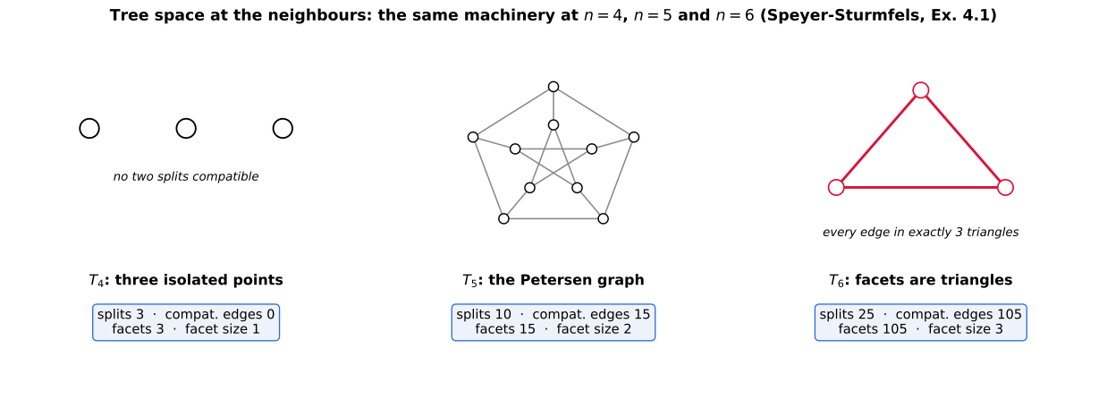
Tree space at n = 4, 5 and 6: three isolated points, the Petersen graph, and triangle facets, each panel with its asserted counts of splits, compatibility edges, facets and facet size

Figure 11.2 — The table above, drawn. Every cell — splits, compatibility edges, facets, facet size, and the n = 6 split types below — was recomputed by the figure script from the chapter program and asserted before rendering.

For n = 6: the 25 splits split as 15 of type 2|4 plus 10 of type 3|3; every facet is a triangle (tree space is pure of dimension 2); every edge lies in exactly 3 triangles; and 105 = 7!! facets, 25 = 2⁵ − 6 − 1 vertices, as Theorem 3.4 predicts. For n = 4 the machinery returns Chapter 10’s answer in this language: 3 splits, no two compatible, G‴_{2,4} = three isolated points.

Predict-first moral. Nothing in §§11.2–11.6 used the number 5 except through the combinatorics of its subsets. That is why the corroboration row matters: a construction that only works at the value it was built for is a coincidence; one that reproduces n = 4 behind it and n = 6 ahead of it is a theorem, running.

Honest Box — the sign typo, one rung up. Chapter 10’s Honest Box recorded that equation (8) of Speyer–Sturmfels prints the cone generators as +E_{A,B}, where the paper’s own four-point condition (6) and its convention “−w_{ij} is the distance” force −E_{A,B}. The correction is not an n = 4 accident: this chapter’s program re-verifies it at n = 5 for every split — −E_A satisfies the four-point condition on all five quadruples, +E_A satisfies it on none of the splits tested (it violates the condition outright). When a typo survives a change of dimension, it is worth having caught it by computation rather than by eye.

11.8 The whole chapter, as a program

Everything in this chapter is one runnable program: ch11_petersen.py — exact Fractions throughout, no dependencies beyond the standard library. Its assertions are the chapter’s claims: splits and the compatibility = disjointness check; the Petersen invariants (including hypohamiltonicity and the complement-of-L(K₅) identification); maximal cliques = facets; exact cone membership and decomposition over ℚ; the lineality rank rank(image φ) = 5 with (1,…,1) = φ(½·1); initial forms of the five Plücker quadrics; the closed-form balancing identity at all ten rays; the Try It 1 and 3 answers; and the n = 4 / n = 6 corroboration. Run it, and if it prints its final line, the claims are what we said they are. (This section used to print the listing inline; a screenful of code you can download is just a download with extra scrolling.)

11.9 Try It

Which splits are compatible with 12|345? List them, and say what each pair {12, B} is, geometrically.
Compute the cycle rank of the Petersen graph from V and E, and state what Theorem 3.4 predicts it should equal. What goes wrong with “three pairwise compatible splits” — in leaf-counting terms?
At the ray point w = −E_{12}, how many of the five Plücker quadrics have binomial initial form, how many trinomial — and which quadruples give the trinomials?
Verify the balancing identity of §11.6 by hand for A = {1,2} on one pair of each of the three kinds (inside A, cross, inside A^c).

Answers

1. The 2-subsets of {3,4,5}: 34, 35, 45. Each pair {12, B} is a facet — a trivalent tree on five leaves whose two internal edges are the splits 12|345 and B|B^c.
2. E − V + 1 = 15 − 10 + 1 = 6 = (5−2)! — the bouquet of six circles in Theorem 3.4. Three pairwise compatible 2|3 splits would need three pairwise disjoint 2-sets: six distinct leaves. There are five.
3. 3 binomial, 2 trinomial. The trinomial quadruples are exactly those meeting {1,2} in one leaf: 1345 and 2345.
4. Neighbours of 12: 34, 35, 45. Pair 12 (inside A): no neighbour cuts it, E_A does not cut it, φ-term 0 — 0 = 0. Cross pair, say 13: cut by neighbours 34 and 35 (contribution 2); right side: E_A cuts it (1) plus 2·φ(½·1_{345}) contributes 2·½ = 1 — 2 = 2. Pair inside A^c, say 34: cut by neighbours 35 and 45 (2); right side: E_A contributes 0, the φ-term contributes 2·1 = 2 — 2 = 2.

What we learned

A famous counterexample is a moduli space. The Petersen graph is T₅: its vertices are the ten splits of five leaves, its edges are the fifteen trivalent trees, and the identification is by construction (Kneser KG(5,2), the complement of L(K₅)), not by resemblance.
The invariants are the proof. Girth 5, diameter 2, chromatic number 3, nonplanarity by the Euler bound, hypohamiltonicity by brute force over all ten deletions, and cycle rank 6 = (5−2)! matching Theorem 3.4’s bouquet of circles — each asserted, several twice.
Balancing can be one identity. At every ray the three neighbouring cut vectors sum to the ray’s own vector plus a lineality term, in closed form, for a three-case counting reason a reader can check with a pencil.

Part V closes here. Part VI turns to chip-firing: take the cycle inside Chapter 3’s cubic — a circle, topologically; the donut of the next chapter’s title is its classical cousin, not the same image — and fire chips on it: its sandpile group is ℤ/6, and the group law is rotation. Chapter 12 builds the sandpile group of a donut.

Source & provenance: Day 11 (2026-10-21) of the tropical geometry study — code hidden_files/code/day11_petersen.py, figure files/figures/day11-petersen-tree-space.png (generator hidden_files/code/day11_figures.py), study log Day 11 entry, run log hidden_files/day11-run.log. Source: D. Speyer & B. Sturmfels, “The tropical Grassmannian”, arXiv:math/0304218 — Ex. 3.3, Thm 3.4, compatibility (4), four-point condition (6), cone presentation (8) with Chapter 10’s sign correction, Ex. 4.1. The chapter program was re-run end-to-end from this bundle on 2026-11-13, all assertion groups passing (run log hidden_files/ch11-run.log), including the Phase-2 additions of 2026-11-12 (complement of L(K₅), lineality rank, hypohamiltonicity, explicit Try It 1 and 3 answers). Figures regenerated as SVG the same day: code hidden_files/code/ch11_extra_figures.py, which imports the chapter program, asserts every value it draws — including every cell of the §11.7 table — and only then renders. Referee pass (Nyx, #minplus-book): her five anchors were checked one by one in Phase 2; four held and were folded in, and the fifth — her 9!! = 105 for the n = 6 facet count — was her slip, as she conceded on 2026-11-12 (9!! = 945; (2·6−5)!! = 7!! = 105 is what §11.7 says and the program asserts); she confirmed nothing blocks Phase 3. Duet’s main referee pass arrived later on 2026-11-13: verdict clean, with five small notes — the two time-sensitive ones (this provenance line and the ‘Next’ bridge above) corrected in a follow-up patch, the rest batched with the Chapter 12 cycle.

Chapter code

The full program behind this chapter, as a download: ch11_petersen.py — the same file §11.8 points at. Its assertions are the chapter’s claims; run it.